Background

I don’t remember when I first heard of Nassim N. Taleb, but I started reading his work a little more than a year ago. I usually struggle to understand some of his ideas or technical work but his work has personally been hard to shake off. I keep returning to his work and over time they tend to start making more and more sense the more I study them. Taleb’s work has been both influential and motivational for me to independently keep studying statistics (and more importantly probability).

Recently, there was a interesting twitter fued between Taleb and Claire Lemon, founder of Quillette. They debated over the scientific validity of IQ. A summary of the events can be found here. From my position, one of the points of contentious by Taleb was the lack of understanding and use of correlation by social scientist, especially with IQ research being entirely built around correlation.

In the midst of the civil conversation on twitter, I saw a video by Taleb talking about the randomness of correlation. In the video he ran through a simple exercise that showed you can randomly take two normally distributed variables and find spurious correlations. The exercise begins around 3:53 below.

In his exercise, we see that we can get spurious correlations (as high as .64 in the video) when we know intuitively they should 0 because they are random samples of independent normal variables. A few days later, I randomly thought why was this exercise done with a sample size of 18. I was curious to see what would happen if you have a larger sample size. I first replicated his exercise with a sample size of 18 and then ran a size of 100 and 1000.

• Note: I did not notice he also did an example with a sample size of 48 until after I replicated the exercise.

Sample Size: 18

n <- 1:1000 # 1000 trials
cors <- list()

# Run simulation
for (i in seq_along(n)) {
  x <- rnorm(18) # sample size 18
  y <- rnorm(18) # Sample size 18
  cors[i] <- cor(x, y)
}

# Table the correlations
cors_table <- enframe(unlist(cors, use.names = TRUE))

# Plot the results
ggplot(cors_table) +
  geom_line(aes(1:1000, value)) +
  scale_y_continuous(limits = c(-1,1)) +
  labs(x = "Trials", 
       y = "Correlation") +
  theme_minimal() +
  theme(
    panel.grid.major.x = element_blank(),
    panel.grid.minor.x = element_blank())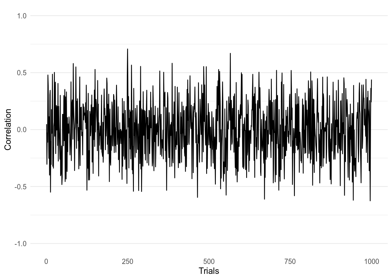

Figure 1: 1000 Correlations taken from two normally distributed variables with a sample size of 18.

We get similar results as Taleb. Over 1000 trials, most of the correlations are bounded within \(\pm .5\). The highest correlations we find on the upper and lower bound are 0.71 and -0.63. This is not what we want to see when these are just random data points from normal distributed variables. Now lets see what happens with a bigger sample size.

Sample Size: 100

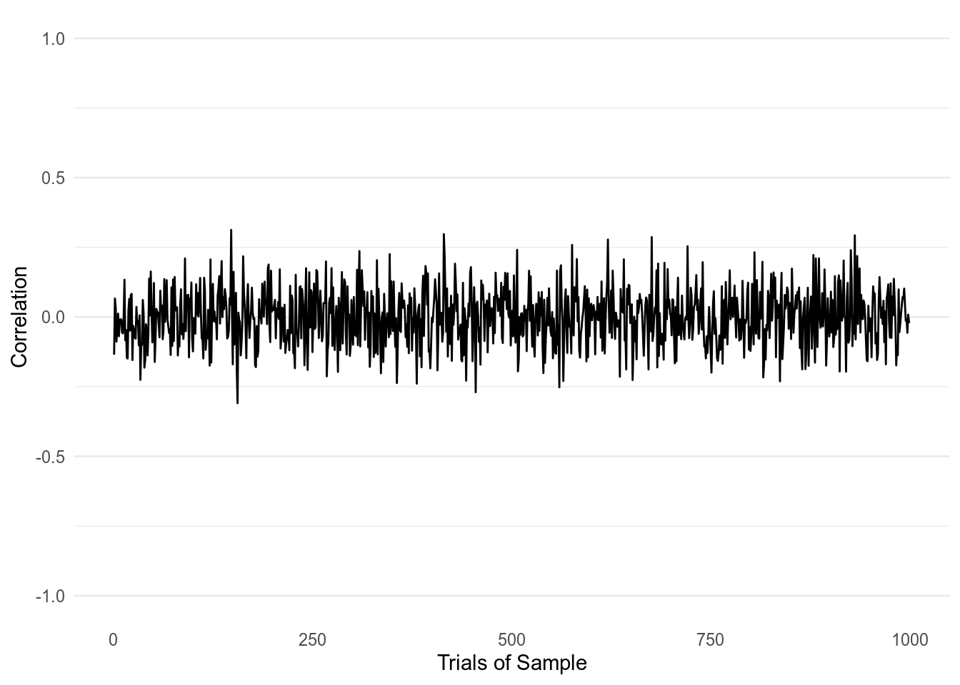
Figure 2: 1000 Correlations taken from two normally distributed variables with a sample size of 100.

With a sample size of 100, the correlations are overall closer to 0, but they are still bounded around \(\pm .25\). The highest correlations we find on the upper and lower bound are 0.31 and -0.31.

Sample Size: 1000

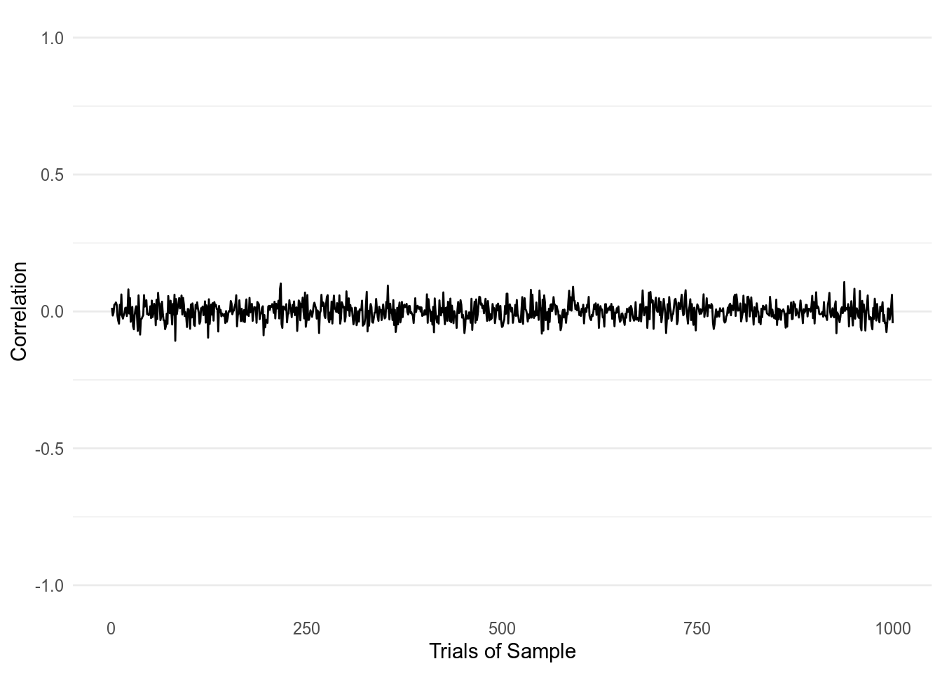
Figure 3: 1000 Correlations taken from two normally distributed variables with a sample size of 1000.

With a sample size of 1000, we finally get correlations that are near 0 as what we should expect. Yet the biggest correlations we get still reach 0.11 and -0.11.

Discussion

Overall, this was a fun exercise to walk through. My personal take away is just to be more cautious with correlations. There might certainly be other issues to consider when using correlations but here we just wanted extend Taleb’s lesson on how easy it is to find spurious correlations.

Returning to the IQ discussion, this exercise can also help put in context the correlations found in IQ studies by their sample size. In a recent post by Sean McClure, a highly-cited study found the average sample-size of IQ studies to be 68. The paper can be found here. However, I want to point out that the paper was published in the 70’s and I hope current IQ research are using larger sample sizes. Yet that still doesn’t take away the historical background of IQ research, especially with the paper mentioning more than 1,500 other IQ studies were examined.